What is Information Retrieval (IR)?

2. The Evolution of Information Retrieval

3. The Information Retrieval Pipeline

At its core, every search engine is an Information Retrieval (IR) system. In this section, we'll break down how that pipeline works. We can divide the process into two stages: the Offline Phase (preparing the data behind the scenes) and the Online Phase (handling the live user query).

Offline Phase (Preparing the Data)

1. Document Collection (Ingestion): Gathering the corpus (e.g., a library of books, a database of products, or crawled web pages) that the system will search through.

2. Document Processing & Cleaning: Standardizing the raw data to extract meaningful text before the system can “read” it.
Strategies include: Cleaning (removing HTML/noise), tokenization (splitting into words), normalization (lowercasing/stemming), and stop-word removal.

3. Defining the IR Model (The Logic): Establishing the foundational framework that dictates how the system views the relationship between documents and queries.
Examples: Boolean model, Vector Space model, or Probabilistic model.

4. Indexing the Documents: Because scanning every document at search time is impossible, the system pre-builds a highly optimized “map” based on the chosen IR model to allow for instant retrieval.
Examples: Inverted indexes (for keyword search) or Vector indexes (for semantic search).

Online Phase (Handling the Search)

5. Query Processing & Understanding: Translating the user's raw input into the language of the index. Strategies include: Applying the exact same cleaning steps used on the documents, query correction (fixing typos), query expansion (adding synonyms), and intent detection.

6. Query Transformation: Applying the IR model's logic to convert the processed query into the exact same “format” as the indexed documents (e.g., turning the query into a vector).

7. Matching and Scoring: The core operation where the system evaluates and sorts the documents.
Matching: Fast retrieval of candidate documents that contain the query terms (often combined with hard metadata filters like date or price).
Scoring: Assigning a numerical weight (Retrieval Status Value) to each matched document.
Examples: TF-IDF (rewards frequent but unique terms), BM25 (handles document length penalties), or Cosine Similarity (for vector search).

8. Ranking & Re-Ranking: Sorting documents by their score. Advanced systems use a fast scorer for the top 1,000 results, then apply a heavier, Machine Learning-based “Re-ranker” to finely sort the top 100.

9. Presentation of Results: Displaying the ranked list to the user, often generating context snippets or highlighting matched keywords.

Optional — Evaluation & Feedback Loop: Tracking user behavior (e.g., clicks, dwell time) or asking “Was this result helpful?” to measure system performance and improve future rankings.

4. IR Models

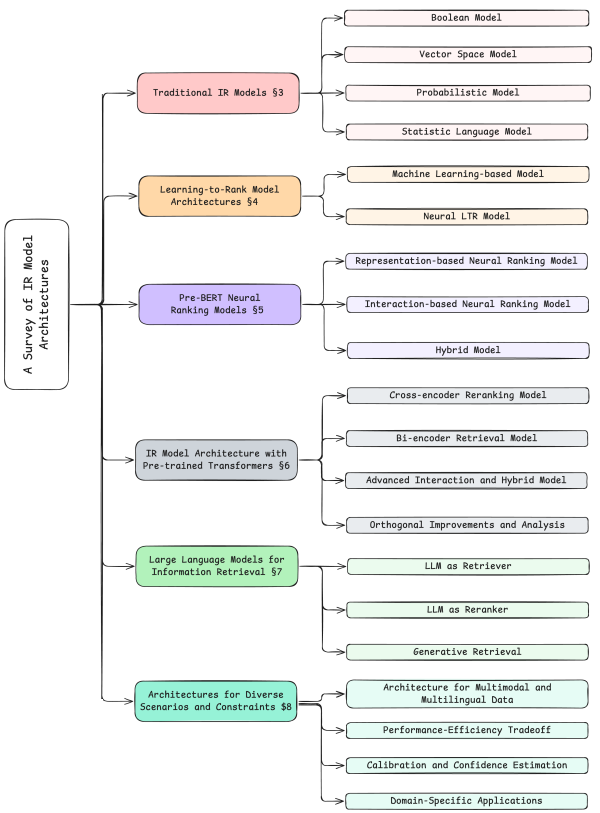
Information Retrieval has evolved dramatically over the decades, moving from basic keyword matching to deep, semantic understanding using Large Language Models. Below is a breakdown of the major families of IR models, how they work, their pros and cons, and the tools that power them.

1. Traditional IR Models
Includes: Boolean Model, Vector Space Model, Probabilistic Model, Statistical Language Models.

Description: These foundational models rely on exact lexical matching. They treat documents and queries as "bags of words" and score relevance based on mathematical principles like term frequency (TF), inverse document frequency (IDF), and probabilistic term distribution. The most famous algorithm in this family is BM25.

What it solves: Extremely fast, efficient, and reliable exact-keyword retrieval. They are great at finding specific names, IDs, or exact phrases in massive collections without needing expensive hardware.

Drawbacks: The "Vocabulary Mismatch Problem." If a user searches for "automobile" but the document says "car," traditional models will fail to match them. They completely lack semantic understanding and context.

Known Tools: Apache Lucene, Elasticsearch, OpenSearch, Apache Solr, Sphinx.

2. Learning-to-Rank (LTR) Model Architectures
Includes: ML-based Models (e.g., LambdaMART, XGBoost), Early Neural LTR Models (e.g., RankNet, ListNet).

Description: Instead of relying on a single scoring formula (like BM25), LTR uses Machine Learning to combine dozens or hundreds of "features" (e.g., keyword match score, document recency, page rank, historical click-through rates) to predict the optimal ranking order of a set of documents.

What it solves: Allows search engines to balance diverse ranking signals—such as textual relevance, business logic (e.g., profit margin), and user behavior—into one highly optimized ranking pipeline.

Drawbacks: Requires massive amounts of high-quality labeled data (like user click logs) to train. It also requires heavy manual "feature engineering" to define what signals the ML model should look at.

Known Tools: XGBoost, LightGBM, Elasticsearch LTR Plugin, RankLib, Metarank.

3. Pre-BERT Neural Ranking Models
Includes: Representation-based Neural Models (e.g., DSSM), Interaction-based Neural Models (e.g., DRMM, KNRM), Hybrid Models (e.g., DUET).

Description: The first wave of deep learning in search. Representation-based models use neural networks to convert queries and documents into embeddings and compare their distance. Interaction-based models compare every word in the query to every word in the document early in the network to find local matching patterns. Hybrid models combine both approaches.

What it solves: They began to bridge the semantic gap and solve the vocabulary mismatch problem without relying on manual feature engineering, learning relationships between words directly from data.

Drawbacks: Because they lacked deep, contextual pre-training on massive datasets (which BERT later introduced), they often struggled to beat highly tuned traditional models (like BM25) on large datasets. They were also computationally heavy for their time.

Known Tools: MatchZoo (a toolkit for deep text matching), historical implementations of Microsoft Bing (which pioneered DSSM).

4. IR Model Architecture with Pre-trained Transformers
Includes: Cross-encoder Reranking, Bi-encoder Retrieval (Dense Retrieval), Advanced Interaction & Hybrid Models (e.g., ColBERT, SPLADE).

Description: The modern era of search powered by Transformers (like BERT). Bi-encoders encode queries and docs independently into dense vectors, matching them via spatial proximity (vector search). Cross-encoders feed both the query and doc into a transformer simultaneously for deep, highly accurate relevance scoring. Advanced Interaction (Late Interaction), like ColBERT, strikes a balance by encoding queries and docs separately but allowing rich word-by-word comparisons during the search.

What it solves: Achieves state-of-the-art semantic understanding. They understand context, phrasing, and synonyms flawlessly (e.g., knowing that "visa" means a travel document in one context and a credit card in another).

Drawbacks: High computational and memory cost. Bi-encoders require specialized Vector Databases to search efficiently and can struggle with out-of-domain terms (like new product names). Cross-encoders are too slow to search an entire database, so they are restricted to re-ranking the top 100 results.

Known Tools: Hugging Face sentence-transformers, Vector Databases (Pinecone, Milvus, Qdrant, Weaviate), Vespa, Faiss.

5. LLMs for IR
Includes: LLM as Retriever, LLM as Reranker, Generative Retrieval.

Description: Leverages large language models (like GPT-4, LLaMA) for search. LLM as Reranker (e.g., RankGPT) prompts an LLM to look at a list of documents and reorder them based on deep reasoning. Generative Retrieval (e.g., Differentiable Search Index) is a radical approach where the LLM memorizes the entire document corpus and directly generates the Document ID as text in response to a query.

What it solves: Offers unparalleled reasoning capabilities for highly complex, multi-faceted queries. They can perform zero-shot retrieval with incredibly high accuracy without needing task-specific training data.

Drawbacks: Exceptionally slow and expensive. API calls or local inference for large LLMs cost significantly more than traditional or BERT-based models. Furthermore, Generative Retrieval struggles with dynamic indexes—adding a new document often requires retraining/fine-tuning the LLM.

Known Tools: OpenAI API, LlamaIndex, LangChain, RankGPT, DSPy.

6. Architectures for Diverse Scenarios and Constraints
Includes: Multilingual Search, Multi-modal IR, Conversational/Session-based Search.

Description: Highly specialized architectures built for specific user experiences. Multilingual models (e.g., mBERT) project multiple languages into a single vector space. Multi-modal models (e.g., CLIP) align text, images, and audio. Conversational search architectures maintain memory and dialogue state across multiple user interactions.

What it solves: Expands search beyond monolingual text boxes. They allow users to search for images using text, search documents in languages they don't speak, or have back-and-forth dialogue with search agents (like ChatGPT's browsing feature).

Drawbacks: Highly complex to deploy. Multi-modal models require perfectly paired training data (e.g., millions of image-caption pairs). Conversational models suffer from "context drift," where the system loses track of the user's original intent over a long conversation.

Known Tools: OpenAI CLIP, Cohere Multilingual Embeddings, Google Vertex AI Search, Apache Lucene (which now supports multi-modal dense vectors).

5. Evaluation Metrics

To know if a search engine is actually good, we have to measure its performance. IR evaluation generally falls into several categories, ranging from basic counting metrics to advanced user-behavior tracking.

1. Set-Based Metrics (Unranked)

These metrics treat the search results as an unordered "basket" of documents. They are generally evaluated at a specific cutoff point (e.g., the top 10 results, written as @K).

Precision (and Precision@K)

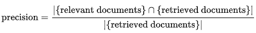
Definition: The percentage of retrieved documents that are actually relevant to the user's query. If we look only at the top 10 results, we call it Precision@10.
Interpretation: Precision answers the question: "Out of the documents the system showed me, how many were actually useful?" A high precision means the system rarely returns "junk" or irrelevant results.

Recall (and Recall@K)

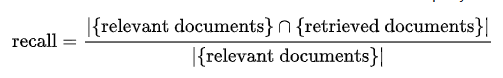
Definition: The percentage of all existing relevant documents in the database that the search system successfully retrieved.
Interpretation: Recall answers the question: "Did the system miss anything important?" A high recall means the system is very thorough. In legal or medical search, high recall is crucial because missing a single document could be disastrous.

F1-Score

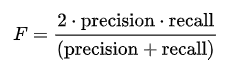
Definition: The harmonic mean of Precision and Recall.
Interpretation: Precision and Recall are usually at odds with each other (if you retrieve more documents to increase recall, your precision usually drops). The F1-Score provides a single, balanced metric that ensures your system isn't severely failing at one at the expense of the other.

2. Rank-Based Metrics (Position-Aware)

Users rarely look past the first page of search results. Therefore, order matters. These metrics evaluate not just if a relevant document was found, but how high up it was placed.

Mean Reciprocal Rank (MRR)

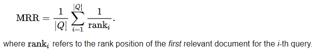
Definition: MRR looks only at the rank of the first relevant document retrieved. It calculates the reciprocal of that rank (1 divided by the rank). If the first relevant doc is at position 1, the score is 1. If it's at position 3, the score is 1/3 (0.33). "Mean" simply averages this score across a sample of queries Q.
Interpretation: MRR answers the question: "How quickly did the user find a right answer?" It is the perfect metric for "Known-Item Search" (like searching for a specific user ID) or Question Answering (QA), where the user only needs one correct answer and doesn't care about the rest of the list.

Mean Average Precision (MAP)

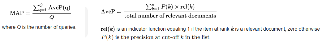
Definition: MAP evaluates the whole ranked list. For a single query, it calculates the Precision at every point a relevant document is found, and then takes the "Average Precision" (AP) of those points. MAP is the mean of these AP scores across many queries.
Interpretation: MAP rewards search engines that put all the relevant documents at the very top. It is a highly robust metric for comprehensive searches where a user wants to see multiple relevant results (e.g., "Show me articles about the 2008 financial crisis").

3. Graded Relevance Metrics

Real-world search isn't just "Relevant vs. Irrelevant" (binary). Some documents are perfect, some are somewhat helpful, and some are useless.

Normalized Discounted Cumulative Gain (NDCG)

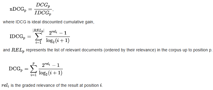
Definition: NDCG assigns a graded score to documents (e.g., 0 = bad, 1 = fair, 2 = good, 3 = perfect).

• Gain: The relevance score of the document.
• Discounted: The score is mathematically reduced (discounted) the further down the list the document appears.
• Cumulative: The discounted scores are added up.
• Normalized: The final score is divided by the "Ideal" ranking (the absolute best possible order) to get a percentage between 0.0 and 1.0.

Interpretation: NDCG is the industry gold standard for evaluating web search engines and e-commerce platforms. It answers the question: "Did the absolute best, most highly relevant documents appear at the very top, with moderately relevant ones below them?"

4. Modern LLM & RAG Metrics

LLM-as-a-Judge (Context Relevance / Precision)

Definition: Instead of relying on human-labeled datasets, a powerful LLM (like GPT-4) is prompted to act as an impartial judge. It reads the user's query and the retrieved documents, and outputs a score based on how well the document contains the exact information needed to answer the query.
Interpretation: Answers the question: "Did we retrieve the exact context an LLM needs to generate a correct answer?" This is widely used in modern RAG frameworks (like Ragas or TruLens) because it is much faster and cheaper than hiring humans to grade search results.

5. Online / User-Behavior Metrics

Click-Through Rate (CTR) & Position Bias

Definition: The ratio of users who click on a specific search result compared to the total number of users who viewed the search page.
Interpretation: A high CTR on the top results implies the search engine is doing a good job. However, engineers must account for Position Bias (users naturally click the first link even if it's bad).

Mean Time to Success (MTTS) & Abandonment Rate

Definition: MTTS measures how long it takes a user to issue a query, click a result, and not return to the search page. Abandonment Rate measures how often users search but leave the page without clicking anything.
Interpretation: If MTTS is low, the search engine is fast and accurate. If the abandonment rate is high, it means the search engine returned unhelpful results, forcing the user to give up.-modal dense vectors).

6. Benchmarks

• BIRCO Benchmark
• BEIR Benchmark

7. Sources

• Zilliz series on Information Retrieval
• Wikipedia - Information Retrieval
• A Survey of Model Architecture in Information Retrieval by Xu et al. (2026)
• Wikipedia - Evaluation Measures for Information Retrieval
• Wikipedia - Discounted Cumulative Gain